Transport distributions using dense solvers

In this example, we sample 2 toy distributions and compute a dense fugw alignment between them. Dense alignments are typically used when both aligned distributions have less than 10k points.

import matplotlib.pyplot as plt
import numpy as np
import torch

from fugw.mappings import FUGW
from fugw.utils import _init_mock_distribution
from matplotlib.collections import LineCollection

torch.manual_seed(0)

n_points_source = 50
n_points_target = 40
n_features_train = 2
n_features_test = 2

Let us generate random training data for the source and target distributions

_, source_features_train, source_geometry, source_embeddings = (
    _init_mock_distribution(n_features_train, n_points_source)
)
_, target_features_train, target_geometry, target_embeddings = (
    _init_mock_distribution(n_features_train, n_points_target)
)
source_features_train.shape

/usr/local/lib/python3.8/site-packages/torch/distributions/wishart.py:272: UserWarning:

Singular sample detected.


torch.Size([2, 50])

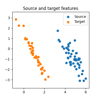
We can visualize the generated features:

fig = plt.figure(figsize=(4, 4))
ax = fig.add_subplot()
ax.set_title("Source and target features")
ax.set_aspect("equal", "datalim")
ax.scatter(source_features_train[0], source_features_train[1], label="Source")
ax.scatter(target_features_train[0], target_features_train[1], label="Target")
ax.legend()
plt.show()

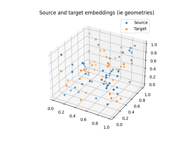
And embeddings:

fig = plt.figure()
ax = fig.add_subplot(projection="3d")
ax.set_title("Source and target embeddings (ie geometries)")
ax.scatter(
    source_embeddings[:, 0],
    source_embeddings[:, 1],
    source_embeddings[:, 2],
    s=15,
    label="Source",
)
ax.scatter(
    target_embeddings[:, 0],
    target_embeddings[:, 1],
    target_embeddings[:, 2],
    s=15,
    label="Target",
)
ax.legend()
plt.show()

Features and geometries should be normalized before calling the solver

source_features_train_normalized = source_features_train / torch.linalg.norm(
    source_features_train, dim=1
).reshape(-1, 1)
target_features_train_normalized = target_features_train / torch.linalg.norm(
    target_features_train, dim=1
).reshape(-1, 1)

source_geometry_normalized = source_geometry / source_geometry.max()
target_geometry_normalized = target_geometry / target_geometry.max()

Let us define the optimization problem to solve

alpha = 0.5
rho = 1000
eps = 1e-4
mapping = FUGW(alpha=alpha, rho=rho, eps=eps)

Now, we fit a transport plan between source and target distributions using a sinkhorn solver

_ = mapping.fit(
    source_features_train_normalized,
    target_features_train_normalized,
    source_geometry=source_geometry_normalized,
    target_geometry=target_geometry_normalized,
    solver="sinkhorn",
    verbose=True,
)

[15:42:09] Validation data for feature maps is not provided. Using  dense.py:199
           training data instead.
           Validation data for anatomical kernels is not provided.  dense.py:226
           Using training data instead.


           BCD step 1/10   FUGW loss:      0.029136842116713524     dense.py:568
           Validation loss:        0.029136842116713524


[15:42:10] BCD step 2/10   FUGW loss:      0.046771109104156494     dense.py:568
           Validation loss:        0.046771109104156494


           BCD step 3/10   FUGW loss:      0.022854337468743324     dense.py:568
           Validation loss:        0.022854337468743324


           BCD step 4/10   FUGW loss:      0.02232404239475727      dense.py:568
           Validation loss:        0.02232404239475727


[15:42:11] BCD step 5/10   FUGW loss:      0.04798972234129906      dense.py:568
           Validation loss:        0.04798972234129906


           BCD step 6/10   FUGW loss:      0.02343880571424961      dense.py:568
           Validation loss:        0.02343880571424961


           BCD step 7/10   FUGW loss:      0.019214436411857605     dense.py:568
           Validation loss:        0.019214436411857605


[15:42:12] BCD step 8/10   FUGW loss:      0.01873275265097618      dense.py:568
           Validation loss:        0.01873275265097618


           BCD step 9/10   FUGW loss:      0.01861358806490898      dense.py:568
           Validation loss:        0.01861358806490898


           BCD step 10/10  FUGW loss:      0.018613653257489204     dense.py:568
           Validation loss:        0.018613653257489204

The transport plan can be accessed after the model has been fitted

pi = mapping.pi
print(f"Transport plan's total mass: {pi.sum():.5f}")

Transport plan's total mass: 0.99999

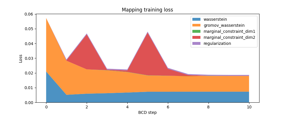
Here is the evolution of the FUGW loss during training, as well as the contribution of each loss term:

fig, ax = plt.subplots(figsize=(10, 4))
ax.set_title("Mapping training loss")
ax.set_ylabel("Loss")
ax.set_xlabel("BCD step")
ax.stackplot(
    mapping.loss_steps,
    [
        (1 - alpha) * np.array(mapping.loss["wasserstein"]),
        alpha * np.array(mapping.loss["gromov_wasserstein"]),
        rho * np.array(mapping.loss["marginal_constraint_dim1"]),
        rho * np.array(mapping.loss["marginal_constraint_dim2"]),
        eps * np.array(mapping.loss["regularization"]),
    ],
    labels=[
        "wasserstein",
        "gromov_wasserstein",
        "marginal_constraint_dim1",
        "marginal_constraint_dim2",
        "regularization",
    ],
    alpha=0.8,
)
ax.legend()
plt.show()

Using the computed mapping

The computed mapping is stored in mapping.pi as a torch.Tensor. In this example, the transport plan is small enough that we can display it altogether.

fig, ax = plt.subplots(figsize=(4, 4))
ax.set_title("Transport plan")
ax.set_xlabel("target vertices")
ax.set_ylabel("source vertices")
im = plt.imshow(pi, cmap="viridis")
plt.colorbar(im, ax=ax, shrink=0.8)
plt.show()

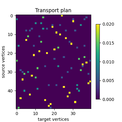
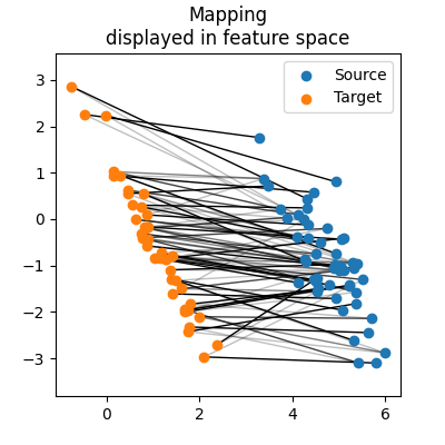
The previous figure of the transport plan tells us it is very sparse and not very regularized. Another informative way to look at the plan consists in checking which points of the source and target distributions were matched together in the feature space.

fig = plt.figure(figsize=(4, 4))
ax = fig.add_subplot()
ax.set_aspect("equal", "datalim")
ax.set_title("Mapping\ndisplayed in feature space")

# Draw lines between matched points
indices = torch.cartesian_prod(
    torch.arange(n_points_source), torch.arange(n_points_target)
)
segments = torch.stack(
    [
        source_features_train[:, indices[:, 0]],
        target_features_train[:, indices[:, 1]],
    ]
).permute(2, 0, 1)
pi_normalized = pi / pi.sum(dim=1).reshape(-1, 1)
line_segments = LineCollection(
    segments, alpha=pi_normalized.flatten(), colors="black", lw=1, zorder=1
)
ax.add_collection(line_segments)

# Draw distributions
ax.scatter(source_features_train[0], source_features_train[1], label="Source")
ax.scatter(target_features_train[0], target_features_train[1], label="Target")

ax.legend()
plt.show()

Finally, the fitted model can transport unseen data between source and target

source_features_test = torch.rand(n_features_test, n_points_source)
target_features_test = torch.rand(n_features_test, n_points_target)
transformed_data = mapping.transform(source_features_test)
transformed_data.shape

torch.Size([2, 40])

assert transformed_data.shape == target_features_test.shape

Estimated memory usage: 127 MB