Note
Go to the end to download the full example code.
Transport distributions using sparse solvers#
In this example, we sample 2 toy distributions and compute a sparse fugw alignment between them. Sparse alignments are typically used when both aligned distributions have more than 10k points.
import matplotlib.pyplot as plt
import numpy as np
import torch

from fugw.mappings import FUGW, FUGWSparse
from fugw.scripts import coarse_to_fine
from fugw.utils import _init_mock_distribution
from matplotlib.collections import LineCollection
from scipy.sparse import coo_matrix
torch.manual_seed(13)

n_points_source = 300
n_samples_source = 100
n_points_target = 300
n_samples_target = 100
n_features_train = 2
n_features_test = 2
Let us generate random training data for the source and target distributions
_, source_features_train, _, source_embeddings = _init_mock_distribution(
    n_features_train, n_points_source
)
_, target_features_train, _, target_embeddings = _init_mock_distribution(
    n_features_train, n_points_target
)
/usr/local/lib/python3.8/site-packages/torch/distributions/wishart.py:272: UserWarning:

Singular sample detected.
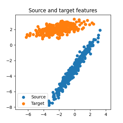
We can visualize the generated features:
fig = plt.figure(figsize=(4, 4))
ax = fig.add_subplot()
ax.set_title("Source and target features")
ax.set_aspect("equal", "datalim")
ax.scatter(source_features_train[0], source_features_train[1], label="Source")
ax.scatter(target_features_train[0], target_features_train[1], label="Target")
ax.legend()
plt.show()
Do not forget to normalize features and embeddings before fitting the models.
source_features_train_normalized = source_features_train / torch.linalg.norm(
    source_features_train, dim=1
).reshape(-1, 1)
target_features_train_normalized = target_features_train / torch.linalg.norm(
    target_features_train, dim=1
).reshape(-1, 1)

source_embeddings_normalized, source_d_max = coarse_to_fine.random_normalizing(
    source_embeddings
)
target_embeddings_normalized, target_d_max = coarse_to_fine.random_normalizing(
    target_embeddings
)
Let us define the coarse and fine-grained optimization problems to solve. We also specify which solver to use at each of the 2 steps:
alpha_coarse = 0.5
rho_coarse = 1
eps_coarse = 1e-4
coarse_mapping = FUGW(alpha=alpha_coarse, rho=rho_coarse, eps=eps_coarse)
coarse_mapping_solver = "mm"
coarse_mapping_solver_params = {
    "tol_uot": 1e-10,
}

alpha_fine = 0.5
rho_fine = 1
eps_fine = 1e-4
fine_mapping = FUGWSparse(alpha=alpha_fine, rho=rho_fine, eps=eps_fine)
fine_mapping_solver = "mm"
fine_mapping_solver_params = {
    "tol_uot": 1e-10,
}
Now, let us fit both the coarse and fine-grained mappings.
The coarse mapping is fitted on a limited number
of points from the source and target distributions,
which we sample randomly in this example.
You should carefully set the source and target selection_radius
as they will greatly affect the sparsity of the computed mappings.
They should usually be set using domain knowledge related to the
distributions you are trying to align.
# Sub-sample source and target distributions
source_sample = torch.randperm(n_points_source)[:n_samples_source]
target_sample = torch.randperm(n_points_target)[:n_samples_target]

_ = coarse_to_fine.fit(
    # Source and target's features and embeddings
    source_features=source_features_train_normalized,
    target_features=target_features_train_normalized,
    source_geometry_embeddings=source_embeddings_normalized,
    target_geometry_embeddings=target_embeddings_normalized,
    # Parametrize step 1 (coarse alignment between source and target)
    source_sample=source_sample,
    target_sample=target_sample,
    coarse_mapping=coarse_mapping,
    coarse_mapping_solver=coarse_mapping_solver,
    coarse_mapping_solver_params=coarse_mapping_solver_params,
    # Parametrize step 2 (selection of pairs of indices present in
    # fine-grained's sparsity mask)
    coarse_pairs_selection_method="topk",
    source_selection_radius=0.5 / source_d_max,
    target_selection_radius=0.5 / target_d_max,
    # Parametrize step 3 (fine-grained alignment)
    fine_mapping=fine_mapping,
    fine_mapping_solver=fine_mapping_solver,
    fine_mapping_solver_params=fine_mapping_solver_params,
    # Misc
    verbose=True,
)
[14:32:03] Validation data for feature maps is not provided. Using  dense.py:199
           training data instead.
           Validation data for anatomical kernels is not provided.  dense.py:226
           Using training data instead.


           BCD step 1/10   FUGW loss:      0.03209492564201355      dense.py:568
           Validation loss:        0.03209492564201355


[14:32:04] BCD step 2/10   FUGW loss:      0.027612239122390747     dense.py:568
           Validation loss:        0.027612239122390747


           BCD step 3/10   FUGW loss:      0.018442563712596893     dense.py:568
           Validation loss:        0.018442563712596893


           BCD step 4/10   FUGW loss:      0.01579628325998783      dense.py:568
           Validation loss:        0.01579628325998783


           BCD step 5/10   FUGW loss:      0.015153789892792702     dense.py:568
           Validation loss:        0.015153789892792702


[14:32:05] BCD step 6/10   FUGW loss:      0.014875941909849644     dense.py:568
           Validation loss:        0.014875941909849644


           BCD step 7/10   FUGW loss:      0.014715257100760937     dense.py:568
           Validation loss:        0.014715257100760937


           BCD step 8/10   FUGW loss:      0.014592343010008335     dense.py:568
           Validation loss:        0.014592343010008335


[14:32:06] BCD step 9/10   FUGW loss:      0.014477252028882504     dense.py:568
           Validation loss:        0.014477252028882504


           BCD step 10/10  FUGW loss:      0.01438036747276783      dense.py:568
           Validation loss:        0.01438036747276783
/github/workspace/src/fugw/scripts/coarse_to_fine.py:358: UserWarning:

Sparse CSR tensor support is in beta state. If you miss a functionality in the sparse tensor support, please submit a feature request to https://github.com/pytorch/pytorch/issues. (Triggered internally at ../aten/src/ATen/SparseCsrTensorImpl.cpp:53.)

           Validation data for feature maps is not provided. Using sparse.py:209
           training data instead.
           Validation data for anatomical kernels is not provided. sparse.py:253
           Using training data instead.


[14:32:08] BCD step 1/10   FUGW loss:      0.02047727443277836     sparse.py:660


[14:32:11] BCD step 2/10   FUGW loss:      0.014399909414350986    sparse.py:660


[14:32:13] BCD step 3/10   FUGW loss:      0.012644448317587376    sparse.py:660


[14:32:16] BCD step 4/10   FUGW loss:      0.011991660110652447    sparse.py:660


[14:32:18] BCD step 5/10   FUGW loss:      0.011676586233079433    sparse.py:660


[14:32:20] BCD step 6/10   FUGW loss:      0.011500303633511066    sparse.py:660


[14:32:23] BCD step 7/10   FUGW loss:      0.011388624086976051    sparse.py:660


[14:32:25] BCD step 8/10   FUGW loss:      0.011310438625514507    sparse.py:660


[14:32:28] BCD step 9/10   FUGW loss:      0.011251626536250114    sparse.py:660


[14:32:31] BCD step 10/10  FUGW loss:      0.011205767281353474    sparse.py:660
Both the coarse and fine-grained transport plans can be accessed after the models have been fitted
print(f"Coarse transport plan's total mass: {coarse_mapping.pi.sum():.5f}")
print(
    "Fine-grained transport plan's total mass:"
    f" {torch.sparse.sum(fine_mapping.pi):.5f}"
)
Coarse transport plan's total mass: 0.99738
Fine-grained transport plan's total mass: 0.99811
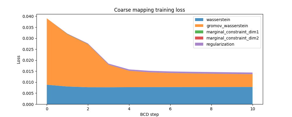
Here is the evolution of the FUGW loss during training of the coarse mapping, as well as the contribution of each loss term:
fig, ax = plt.subplots(figsize=(10, 4))
ax.set_title("Coarse mapping training loss")
ax.set_ylabel("Loss")
ax.set_xlabel("BCD step")
ax.stackplot(
    coarse_mapping.loss_steps,
    [
        (1 - alpha_coarse) * np.array(coarse_mapping.loss["wasserstein"]),
        alpha_coarse * np.array(coarse_mapping.loss["gromov_wasserstein"]),
        rho_coarse * np.array(coarse_mapping.loss["marginal_constraint_dim1"]),
        rho_coarse * np.array(coarse_mapping.loss["marginal_constraint_dim2"]),
        eps_coarse * np.array(coarse_mapping.loss["regularization"]),
    ],
    labels=[
        "wasserstein",
        "gromov_wasserstein",
        "marginal_constraint_dim1",
        "marginal_constraint_dim2",
        "regularization",
    ],
    alpha=0.8,
)
ax.legend()
plt.show()
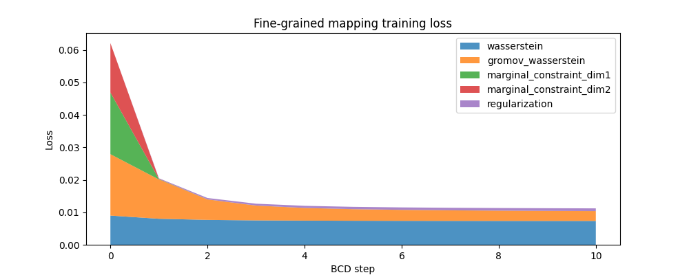
And here is a similar plot for the fine-grained mapping:
fig, ax = plt.subplots(figsize=(10, 4))
ax.set_title("Fine-grained mapping training loss")
ax.set_ylabel("Loss")
ax.set_xlabel("BCD step")
ax.stackplot(
    fine_mapping.loss_steps,
    [
        (1 - alpha_fine) * np.array(fine_mapping.loss["wasserstein"]),
        alpha_fine * np.array(fine_mapping.loss["gromov_wasserstein"]),
        rho_fine * np.array(fine_mapping.loss["marginal_constraint_dim1"]),
        rho_fine * np.array(fine_mapping.loss["marginal_constraint_dim2"]),
        eps_fine * np.array(fine_mapping.loss["regularization"]),
    ],
    labels=[
        "wasserstein",
        "gromov_wasserstein",
        "marginal_constraint_dim1",
        "marginal_constraint_dim2",
        "regularization",
    ],
    alpha=0.8,
)
ax.legend()
plt.show()
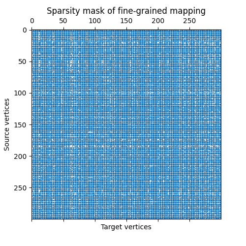
In this example, the computed sparse transport plan is not very sparse: it stores about 60% of what the equivalent dense transport plan would store. When aligning distributions with a high number of points, we usually want to keep this number much smaller.
sparsity_ratio = (
    100 * fine_mapping.pi.values().shape[0] / fine_mapping.pi.shape.numel()
)
print(f"Ratio of non-null coefficients: {sparsity_ratio:.2f}%")
Ratio of non-null coefficients: 86.10%
We can also have a look at the sparsity mask of the fine-grained transport plan. In this particular example, we don’t expect it to show a particularly meaningful structure.
indices = fine_mapping.pi.indices()
fine_mapping_as_scipy_coo = coo_matrix(
    (
        fine_mapping.pi.values(),
        (indices[0], indices[1]),
    ),
    shape=fine_mapping.pi.size(),
)

fig, ax = plt.subplots(figsize=(5, 5))
ax.set_title("Sparsity mask of fine-grained mapping")
ax.set_ylabel("Source vertices")
ax.set_xlabel("Target vertices")
plt.spy(fine_mapping_as_scipy_coo, precision="present", markersize=0.3)
plt.show()
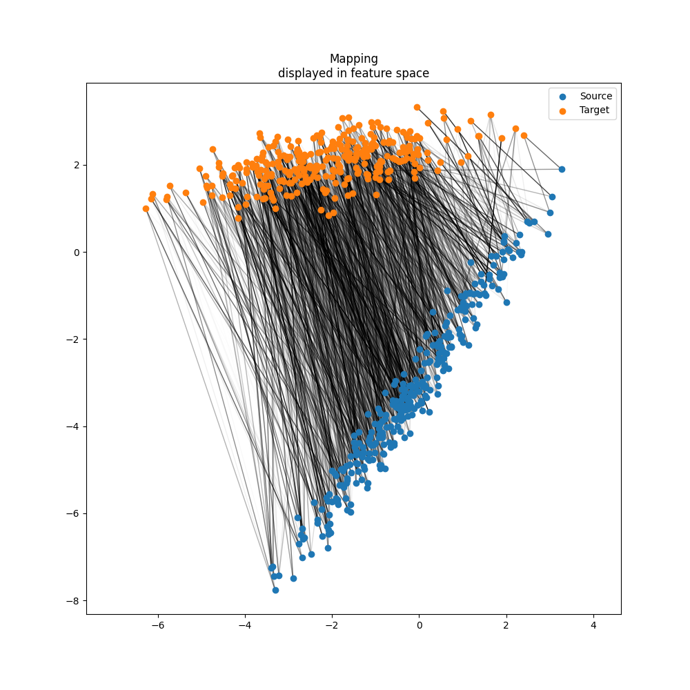
We can observe the computed mappings between source and target points in the feature space.
pi = fine_mapping.pi.to_dense()
fig = plt.figure(figsize=(10, 10))
ax = fig.add_subplot()
ax.set_aspect("equal", "datalim")
ax.set_title("Mapping\ndisplayed in feature space")

# Draw lines between matched points
indices = torch.cartesian_prod(
    torch.arange(n_points_source), torch.arange(n_points_target)
)
segments = torch.stack(
    [
        source_features_train[:, indices[:, 0]],
        target_features_train[:, indices[:, 1]],
    ]
).permute(2, 0, 1)
pi_normalized = pi / pi.sum(dim=1).reshape(-1, 1)
line_segments = LineCollection(
    segments,
    alpha=pi_normalized.flatten().nan_to_num(),
    colors="black",
    lw=1,
    zorder=1,
)
ax.add_collection(line_segments)

# Draw distributions
ax.scatter(source_features_train[0], source_features_train[1], label="Source")
ax.scatter(target_features_train[0], target_features_train[1], label="Target")

ax.legend()
plt.show()
Finally, the fitted fine-grained model can transport unseen data between source and target
source_features_test = torch.rand(n_features_test, n_points_source)
target_features_test = torch.rand(n_features_test, n_points_target)
transformed_data = fine_mapping.transform(source_features_test)
transformed_data.shape
torch.Size([2, 300])
assert transformed_data.shape == target_features_test.shape
Total running time of the script: (0 minutes 34.909 seconds)
Estimated memory usage: 215 MB