High-resolution volume alignment of 2 individuals with fMRI data

In this example, we align 2 low-resolution brain volumes using 4 fMRI feature maps (z-score contrast maps).

import numpy as np
import matplotlib.colors as colors
import matplotlib.pyplot as plt

from mpl_toolkits.axes_grid1 import make_axes_locatable
from nilearn import datasets, image
from fugw.mappings import FUGW, FUGWSparse
from fugw.scripts import coarse_to_fine, lmds

We first fetch 5 contrasts for each subject from the localizer dataset.

n_subjects = 2

contrasts = [
    "sentence reading vs checkerboard",
    "sentence listening",
    "calculation vs sentences",
    "left vs right button press",
    "checkerboard",
]
n_training_contrasts = 4

brain_data = datasets.fetch_localizer_contrasts(
    contrasts,
    n_subjects=n_subjects,
    get_anats=True,
)

source_imgs_paths = brain_data["cmaps"][0 : len(contrasts)]
target_imgs_paths = brain_data["cmaps"][len(contrasts) : 2 * len(contrasts)]

source_im = image.load_img(source_imgs_paths)
target_im = image.load_img(target_imgs_paths)

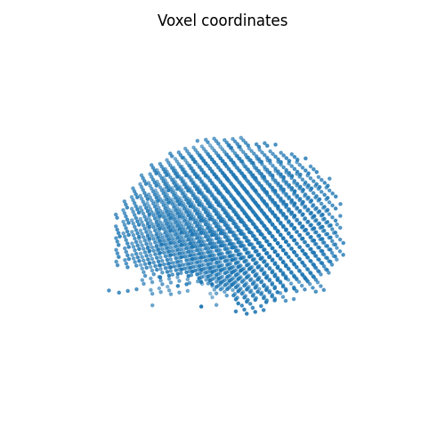
Let’s use a resolution of 2000 voxels so that computations can easily run on a single CPU.

SCALE_FACTOR = 3

source_maps = np.nan_to_num(
    source_im.get_fdata()[::SCALE_FACTOR, ::SCALE_FACTOR, ::SCALE_FACTOR]
)
target_maps = np.nan_to_num(
    target_im.get_fdata()[::SCALE_FACTOR, ::SCALE_FACTOR, ::SCALE_FACTOR]
)

segmentation_fine = np.logical_not(np.isnan(source_im.get_fdata()[:, :, :, 0]))
segmentation_coarse = segmentation_fine[
    ::SCALE_FACTOR, ::SCALE_FACTOR, ::SCALE_FACTOR
]
coordinates = np.array(np.nonzero(segmentation_coarse)).T

source_features = source_maps[
    coordinates[:, 0], coordinates[:, 1], coordinates[:, 2]
].T
target_features = target_maps[
    coordinates[:, 0], coordinates[:, 1], coordinates[:, 2]
].T
source_features.shape

(5, 2258)

fig = plt.figure(figsize=(5, 5))

ax = fig.add_subplot(projection="3d")
ax.set_title("Voxel coordinates")
ax.scatter(coordinates[:, 0], coordinates[:, 1], coordinates[:, 2], marker=".")

ax.view_init(10, 135)
ax.set_axis_off()
plt.tight_layout()
plt.show()

We then compute the distance matrix between voxel coordinates.

source_geometry_embeddings = lmds.compute_lmds_volume(
    segmentation_coarse
).nan_to_num()
target_geometry_embeddings = source_geometry_embeddings.clone()

# Show the embedding shape
print(source_geometry_embeddings.shape)

torch.Size([2258, 3])

In order to avoid numerical errors when fitting the mapping, we normalize both the features and the geometry.

source_features_normalized = source_features / np.linalg.norm(
    source_features, axis=1
).reshape(-1, 1)
target_features_normalized = target_features / np.linalg.norm(
    target_features, axis=1
).reshape(-1, 1)

source_embeddings_normalized, source_distance_max = (
    coarse_to_fine.random_normalizing(source_geometry_embeddings)
)
target_embeddings_normalized, target_distance_max = (
    coarse_to_fine.random_normalizing(target_geometry_embeddings)
)

We now fit the mapping using the sinkhorn solver and 3 BCD iterations.

alpha_coarse = 0.5
rho_coarse = 1
eps_coarse = 1e-4
coarse_mapping = FUGW(alpha=alpha_coarse, rho=rho_coarse, eps=eps_coarse)
coarse_mapping_solver = "mm"
coarse_mapping_solver_params = {
    "nits_bcd": 5,
    "tol_uot": 1e-10,
}

alpha_fine = 0.5
rho_fine = 1
eps_fine = 1e-4
fine_mapping = FUGWSparse(alpha=alpha_fine, rho=rho_fine, eps=eps_fine)
fine_mapping_solver = "mm"
fine_mapping_solver_params = {
    "nits_bcd": 3,
    "tol_uot": 1e-10,
}

Let’s subsample the vertices.

source_sample = coarse_to_fine.sample_volume_uniformly(
    segmentation_coarse,
    embeddings=source_geometry_embeddings,
    n_samples=1000,
)
target_sample = coarse_to_fine.sample_volume_uniformly(
    segmentation_coarse,
    embeddings=target_geometry_embeddings,
    n_samples=1000,
)

/usr/local/lib/python3.8/site-packages/sklearn/cluster/_agglomerative.py:304: UserWarning:

the number of connected components of the connectivity matrix is 3 > 1. Completing it to avoid stopping the tree early.

/usr/local/lib/python3.8/site-packages/sklearn/cluster/_agglomerative.py:304: UserWarning:

the number of connected components of the connectivity matrix is 3 > 1. Completing it to avoid stopping the tree early.

Train both the coarse and the fine mapping. We set the selection radius to 3mm for both source and target (don’t forget to divide by the distance returned by coarse_to_fine.random_normalizing() so that geometries and selection radia have the same units).

_ = coarse_to_fine.fit(
    # Source and target's features and embeddings
    source_features=source_features_normalized[:n_training_contrasts, :],
    target_features=target_features_normalized[:n_training_contrasts, :],
    source_geometry_embeddings=source_embeddings_normalized,
    target_geometry_embeddings=target_embeddings_normalized,
    # Parametrize step 1 (coarse alignment between source and target)
    source_sample=source_sample,
    target_sample=target_sample,
    coarse_mapping=coarse_mapping,
    coarse_mapping_solver=coarse_mapping_solver,
    coarse_mapping_solver_params=coarse_mapping_solver_params,
    # Parametrize step 2 (selection of pairs of indices present in
    # fine-grained's sparsity mask)
    coarse_pairs_selection_method="topk",
    source_selection_radius=3 / source_distance_max,
    target_selection_radius=3 / target_distance_max,
    # Parametrize step 3 (fine-grained alignment)
    fine_mapping=fine_mapping,
    fine_mapping_solver=fine_mapping_solver,
    fine_mapping_solver_params=fine_mapping_solver_params,
    # Misc
    verbose=True,
)

[14:09:52] Validation data for feature maps is not provided. Using  dense.py:202
           training data instead.
           Validation data for anatomical kernels is not provided.  dense.py:229
           Using training data instead.


[14:09:59] BCD step 1/5    FUGW loss:      0.023749656975269318     dense.py:568
           Validation loss:        0.023749656975269318


[14:10:05] BCD step 2/5    FUGW loss:      0.019920265302062035     dense.py:568
           Validation loss:        0.019920265302062035


[14:10:11] BCD step 3/5    FUGW loss:      0.011780289933085442     dense.py:568
           Validation loss:        0.011780289933085442


[14:10:17] BCD step 4/5    FUGW loss:      0.00605743145570159      dense.py:568
           Validation loss:        0.00605743145570159


[14:10:24] BCD step 5/5    FUGW loss:      0.004680723417550325     dense.py:568
           Validation loss:        0.004680723417550325
           Validation data for feature maps is not provided. Using sparse.py:213
           training data instead.
           Validation data for anatomical kernels is not provided. sparse.py:257
           Using training data instead.


[14:10:51] BCD step 1/3    FUGW loss:      0.007941684685647488    sparse.py:660


[14:11:17] BCD step 2/3    FUGW loss:      0.005435771308839321    sparse.py:660


[14:11:44] BCD step 3/3    FUGW loss:      0.004494884517043829    sparse.py:660

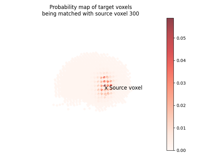
Let’s plot the probability map of target voxels being matched with the 300th source voxel.

pi = fine_mapping.pi
vertex_index = 300
one_hot = np.zeros(source_features.shape[1])
one_hot[vertex_index] = 1.0
probability_map = fine_mapping.inverse_transform(one_hot)

fig = plt.figure(figsize=(7, 5))

ax = fig.add_subplot(projection="3d")
ax.set_title(
    "Probability map of target voxels\n"
    f"being matched with source voxel {vertex_index}"
)

s = ax.scatter(
    coordinates[:, 0],
    coordinates[:, 1],
    coordinates[:, 2],
    marker="o",
    c=probability_map,
    alpha=0.75,
    cmap="Reds",
)

ax.text(
    coordinates[vertex_index, 0],
    coordinates[vertex_index, 1],
    coordinates[vertex_index, 2] - 2,
    "x Source voxel",
    color="black",
    size=12,
)

colorbar = fig.colorbar(s, ax=ax, alpha=1)
colorbar.ax.set_position([0.9, 0.15, 0.03, 0.7])

ax.view_init(10, 135, 2)
ax.set_axis_off()
plt.tight_layout()
plt.show()

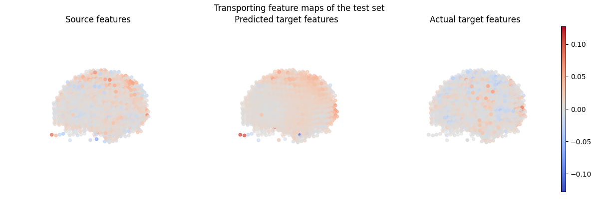
We can now align test contrasts using the fitted fine mapping.

contrast_index = -1
predicted_target_features = fine_mapping.transform(
    source_features[contrast_index, :]
)
predicted_target_features.shape

(2258,)

Let’s compare the Pearson correlation between source and target features.

corr_pre_mapping = np.corrcoef(
    source_features[contrast_index, :], target_features[contrast_index, :]
)[0, 1]
corr_post_mapping = np.corrcoef(
    predicted_target_features, target_features[contrast_index, :]
)[0, 1]
print(f"Pearson Correlation pre-mapping: {corr_pre_mapping:.2f}")
print(f"Pearson Correlation post-mapping: {corr_post_mapping:.2f}")
print(
    "Relative improvement:"
    f" {(corr_post_mapping - corr_pre_mapping) / corr_pre_mapping *100 :.2f} %"
)

Pearson Correlation pre-mapping: 0.38
Pearson Correlation post-mapping: 0.47
Relative improvement: 24.77 %

Let’s plot the transporting feature maps of the test set.

fig = plt.figure(figsize=(12, 4))
fig.suptitle("Transporting feature maps of the test set")

ax = fig.add_subplot(1, 3, 1, projection="3d")
s = ax.scatter(
    coordinates[:, 0],
    coordinates[:, 1],
    coordinates[:, 2],
    marker="o",
    c=source_features_normalized[-1, :],
    cmap="coolwarm",
    norm=colors.CenteredNorm(),
)
ax.view_init(10, 135, 2)
ax.set_title("Source features")
ax.set_axis_off()

ax = fig.add_subplot(1, 3, 2, projection="3d")
ax.scatter(
    coordinates[:, 0],
    coordinates[:, 1],
    coordinates[:, 2],
    marker="o",
    c=predicted_target_features,
    cmap="coolwarm",
    norm=colors.CenteredNorm(),
)
ax.view_init(10, 135, 2)
ax.set_title("Predicted target features")
ax.set_axis_off()

ax = fig.add_subplot(1, 3, 3, projection="3d")
ax.scatter(
    coordinates[:, 0],
    coordinates[:, 1],
    coordinates[:, 2],
    marker="o",
    c=target_features_normalized[-1, :],
    cmap="coolwarm",
    norm=colors.CenteredNorm(),
)
ax.view_init(10, 135, 2)
ax.set_title("Actual target features")
ax.set_axis_off()

ax = fig.add_subplot(1, 1, 1)
ax.set_axis_off()
divider = make_axes_locatable(ax)
cax = divider.append_axes("right", size="1%")
fig.colorbar(s, cax=cax)

plt.tight_layout()
plt.show()

Estimated memory usage: 36 MB