High-resolution surface alignment of 2 individuals with fMRI data

In this example, we show how to use this package to align 2 high-resolution left hemispheres using fMRI feature maps (z-score contrast maps). Note that, since we want this example to run on CPU, we stick to rather low-resolution meshes (around 10k vertices per hemisphere) but that this package can easily scale to resolutions above 150k vertices per hemisphere. In this case, with appropriate hyper-parameters and solver parameters, it takes less than 10 minutes to compute a mapping between 2 such distributions using a V100 Nvidia GPU.

Before reading this tutorial, you should first go through the example aligning brain data at a low-resolution, which explains the ropes of brain alignment in more detail than this example. In the current example, we focus more on how to use this package to align data using real-life resolutions.

import copy
import time

import matplotlib as mpl
import matplotlib.gridspec as gridspec
import matplotlib.pyplot as plt
import numpy as np
import torch

from fugw.mappings import FUGW, FUGWSparse
from fugw.scripts import coarse_to_fine, lmds
from mpl_toolkits.axes_grid1 import make_axes_locatable
from nilearn import datasets, image, plotting, surface
from nilearn.plotting.surf_plotting import CAMERAS, LAYOUT
from plotly.subplots import make_subplots
from scipy.sparse import coo_matrix

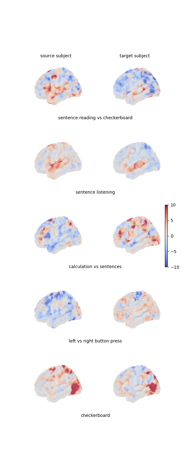
Let’s download 5 volumetric contrast maps per individual using nilearn’s API. We will use the first 4 of them to compute an alignment between the source and target subjects, and use the left-out contrast to assess the quality of our alignment.

np.random.seed(0)
torch.manual_seed(0)

n_subjects = 2

contrasts = [
    "sentence reading vs checkerboard",
    "sentence listening",
    "calculation vs sentences",
    "left vs right button press",
    "checkerboard",
]
n_training_contrasts = 4

brain_data = datasets.fetch_localizer_contrasts(
    contrasts,
    n_subjects=n_subjects,
    get_anats=True,
)

source_imgs_paths = brain_data["cmaps"][0 : len(contrasts)]
target_imgs_paths = brain_data["cmaps"][len(contrasts) : 2 * len(contrasts)]

Computing feature arrays

Let’s project these 4 maps to a mesh of the cortical surface and aggregate these projections to build an array of features for the source and target subjects. For the sake of keeping the training phase of our mapping short even on CPU, we project these volumetric maps on a low-resolution mesh made of 10242 vertices.

fsaverage5 = datasets.fetch_surf_fsaverage(mesh="fsaverage5")

def load_images_and_project_to_surface(image_paths):
    """Util function for loading and projecting volumetric images."""
    images = [image.load_img(img) for img in image_paths]
    surface_images = [
        np.nan_to_num(surface.vol_to_surf(img, fsaverage5.pial_left))
        for img in images
    ]

    return np.stack(surface_images)


source_features = load_images_and_project_to_surface(source_imgs_paths)
target_features = load_images_and_project_to_surface(target_imgs_paths)
source_features.shape

/usr/local/lib/python3.8/site-packages/nilearn/surface/surface.py:464: RuntimeWarning:

Mean of empty slice

/usr/local/lib/python3.8/site-packages/nilearn/surface/surface.py:464: RuntimeWarning:

Mean of empty slice

/usr/local/lib/python3.8/site-packages/nilearn/surface/surface.py:464: RuntimeWarning:

Mean of empty slice

/usr/local/lib/python3.8/site-packages/nilearn/surface/surface.py:464: RuntimeWarning:

Mean of empty slice

/usr/local/lib/python3.8/site-packages/nilearn/surface/surface.py:464: RuntimeWarning:

Mean of empty slice

/usr/local/lib/python3.8/site-packages/nilearn/surface/surface.py:464: RuntimeWarning:

Mean of empty slice

/usr/local/lib/python3.8/site-packages/nilearn/surface/surface.py:464: RuntimeWarning:

Mean of empty slice

/usr/local/lib/python3.8/site-packages/nilearn/surface/surface.py:464: RuntimeWarning:

Mean of empty slice

/usr/local/lib/python3.8/site-packages/nilearn/surface/surface.py:464: RuntimeWarning:

Mean of empty slice

/usr/local/lib/python3.8/site-packages/nilearn/surface/surface.py:464: RuntimeWarning:

Mean of empty slice


(5, 10242)

Here is a figure showing the 4 projected maps for each of the 2 individuals:

def plot_surface_map(
    surface_map, cmap="coolwarm", colorbar=True, engine="matplotlib", **kwargs
):
    """Util function for plotting surfaces."""
    return plotting.plot_surf(
        fsaverage5.pial_left,
        surface_map,
        cmap=cmap,
        colorbar=colorbar,
        bg_map=fsaverage5.sulc_left,
        bg_on_data=True,
        darkness=0.5,
        engine=engine,
        **kwargs,
    )


fig = plt.figure(figsize=(3 * n_subjects, 3 * len(contrasts)))
grid_spec = gridspec.GridSpec(len(contrasts), n_subjects, figure=fig)

# Print all feature maps
for i, contrast_name in enumerate(contrasts):
    for j, features in enumerate([source_features, target_features]):
        ax = fig.add_subplot(grid_spec[i, j], projection="3d")
        plot_surface_map(
            features[i, :], axes=ax, vmax=10, vmin=-10, colorbar=False
        )

    # Add labels to subplots
    if i == 0:
        for j in range(2):
            ax = fig.add_subplot(grid_spec[i, j])
            ax.axis("off")
            ax.text(
                0.5,
                1,
                "source subject" if j == 0 else "target subject",
                va="center",
                ha="center",
            )

    ax = fig.add_subplot(grid_spec[i, :])
    ax.axis("off")
    ax.text(0.5, 0, contrast_name, va="center", ha="center")

# Add colorbar
ax = fig.add_subplot(grid_spec[2, :])
ax.axis("off")
divider = make_axes_locatable(ax)
cax = divider.append_axes("right", size="2%")
fig.add_axes(cax)
fig.colorbar(
    mpl.cm.ScalarMappable(
        norm=mpl.colors.Normalize(vmin=-10, vmax=10), cmap="coolwarm"
    ),
    cax=cax,
)

plt.show()

Estimating geometry kernel matrices

This time, let’s assume matrices of size (n, n) (or (n, m), (m, m)) won’t fit in memory, even with a powerful GPU - as a rule of thumb, this will typically be the case if n is greater than 50k. Therefore, the source and target geometry matrices cannot be explicitly computed. Instead, we derive an embedding X in dimension k to approximate these matrices. Under the hood, this embedding approximates the geodesic distance between all pairs of vertices by computing the true geodesic distance to n_landmarks vertices that are randomly sampled. Higher values of n_landmarks lead to more precise embeddings, although they will take more time to compute. Note that this does not affect the speed of the rest of the alignment procedure, so you might want to invest computational time in deriving precise embeddings. Moreover, this step can easily be parallelized on CPUs.

(coordinates, triangles) = surface.load_surf_mesh(fsaverage5.pial_left)
fs5_pial_left_geometry_embeddings = lmds.compute_lmds_mesh(
    coordinates,
    triangles,
    n_landmarks=100,
    k=3,
    n_jobs=2,
    verbose=True,
)
source_geometry_embeddings = fs5_pial_left_geometry_embeddings
target_geometry_embeddings = fs5_pial_left_geometry_embeddings
source_geometry_embeddings.shape

  100% Geodesic distances (landmarks) ━━━━━━━━━━━━━━━━ 100/100 0:00:07 < 0:00:00

torch.Size([10242, 3])

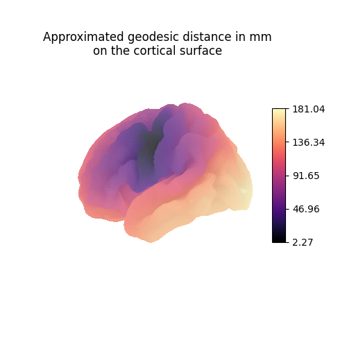
Each line vertex_index of the geometry matrices contains the anatomical distance (here in millimeters) from vertex_index to all other vertices of the mesh.

vertex_index = 12

fig = plt.figure(figsize=(5, 5))
ax = fig.add_subplot(111, projection="3d")
ax.set_title("Approximated geodesic distance in mm\non the cortical surface")
plot_surface_map(
    np.linalg.norm(
        source_geometry_embeddings
        - source_geometry_embeddings[vertex_index, :],
        axis=1,
    ),
    cmap="magma",
    cbar_tick_format="%.2f",
    axes=ax,
)
plt.show()

Normalizing features and geometries

Features and embeddings should be normalized before we can train a mapping. Normalizing embeddings can be tricky, so we provide an empirical method to perform this operation: coarse_to_fine.random_normalizing() samples pairs of indices in the embeddings vector and computes their L2 norm. Eventually, it divides the embeddings vector by the maximum norm it found in this process.

source_features_normalized = source_features / np.linalg.norm(
    source_features, axis=1
).reshape(-1, 1)
target_features_normalized = target_features / np.linalg.norm(
    target_features, axis=1
).reshape(-1, 1)

source_embeddings_normalized, source_distance_max = (
    coarse_to_fine.random_normalizing(source_geometry_embeddings)
)
target_embeddings_normalized, target_distance_max = (
    coarse_to_fine.random_normalizing(target_geometry_embeddings)
)

Training the mapping

Let’s create our mappings. We will need 2 of them: one for computing an alignment between sub-samples of the source and target individuals, the other one for computing a fine-grained alignment leveraging information gathered during the coarse step. Note that the 2 solvers can use different parameters.

alpha_coarse = 0.5
rho_coarse = 1
eps_coarse = 1e-4
coarse_mapping = FUGW(alpha=alpha_coarse, rho=rho_coarse, eps=eps_coarse)
coarse_mapping_solver = "mm"
coarse_mapping_solver_params = {
    "nits_bcd": 5,
    "tol_uot": 1e-10,
}

alpha_fine = 0.5
rho_fine = 1e-2
eps_fine = 1e-4
fine_mapping = FUGWSparse(alpha=alpha_fine, rho=rho_fine, eps=eps_fine)
fine_mapping_solver = "mm"
fine_mapping_solver_params = {
    "nits_bcd": 3,
    "tol_uot": 1e-10,
}

Before fitting our mappings, we sub-sample vertices from the source and target distributions. We could sample them randomly, but a poor sampling of some cortical areas can have really bad consequences on the fine-grained mapping. Therefore, we try to sample vertices uniformly spread across the cortical surface. We use a util function which leverages the ward algorithm to compute this sampling.

source_sample = coarse_to_fine.sample_mesh_uniformly(
    coordinates,
    triangles,
    embeddings=source_geometry_embeddings,
    n_samples=1000,
)
target_sample = coarse_to_fine.sample_mesh_uniformly(
    coordinates,
    triangles,
    embeddings=target_geometry_embeddings,
    n_samples=1000,
)

Let’s inspect the sampled vertices used to derive the coarse mapping. We here switch to plotly to generate interactive figures.

source_sampled_surface = np.zeros(source_features.shape[1])
source_sampled_surface[source_sample] = 1
target_sampled_surface = np.zeros(target_features.shape[1])
target_sampled_surface[target_sample] = 1

# Generate figure with 2 subplots
fig = make_subplots(
    rows=1,
    cols=2,
    specs=[[{"type": "surface"}, {"type": "surface"}]],
    subplot_titles=["Source subject", "Target subject"],
)

fig_source = plot_surface_map(
    source_sampled_surface, cmap="Blues", engine="plotly"
)
fig_target = plot_surface_map(
    target_sampled_surface, cmap="Blues", engine="plotly"
)
fig.add_trace(fig_source.figure.data[0], row=1, col=1)
fig.add_trace(fig_target.figure.data[0], row=1, col=2)

# Edit figure layout
layout = copy.deepcopy(LAYOUT)
m = 50
layout["margin"] = {"l": m, "r": m, "t": m, "b": m, "pad": 0}
layout["scene"]["camera"] = CAMERAS["left"]
layout["scene"]["camera"]["eye"] = {"x": -1.5, "y": 0, "z": 0}
layout["scene2"] = layout["scene"]

fig.update_layout(
    **layout, height=400, width=800, title_text="Sampled vertices", title_x=0.5
)

fig

The rationale behind sampling uniformly across the cortical surface is that only vertices which are within a certain radius of sub-sampled vertices will eventually appear in the sparsity mask, and therefore in the transport plan. In other words, vertices which are too far from sub-sampled vertices won’t be mapped. Let us set a radius of 7 millimeters to see what proportion of vertices will be allowed to be transported. We leverage the properties of sparse matrices to derive a scalable way to derive which vertices are selected.

source_selection_radius = 7
n_neighbourhoods_per_vertex_source = (
    torch.sparse.sum(
        coarse_to_fine.get_neighbourhood_matrix(
            source_geometry_embeddings, source_sample, source_selection_radius
        ),
        dim=1,
    )
    .to_dense()
    .numpy()
)

target_selection_radius = 7
n_neighbourhoods_per_vertex_target = (
    torch.sparse.sum(
        coarse_to_fine.get_neighbourhood_matrix(
            target_geometry_embeddings, target_sample, target_selection_radius
        ),
        dim=1,
    )
    .to_dense()
    .numpy()
)

Let’s now check which vertices will appear in the sparsity mask. In the following figure, deep blue is for vertices which were sampled, light blue for vertices which are within radius-distance of a sampled vertex. Vertices which won’t be selected appear in white. The following figure is interactive. Note that, because embeddings are not very precise for short distances, vertices that are very close to sampled vertices can actually be absent from the mask. In order to limit this effect, the radius should generally be set to a high enough value.

source_vertices_in_mask = np.zeros(source_features.shape[1])
source_vertices_in_mask[n_neighbourhoods_per_vertex_source > 0] = 1
source_vertices_in_mask[source_sample] = 2
target_vertices_in_mask = np.zeros(target_features.shape[1])
target_vertices_in_mask[n_neighbourhoods_per_vertex_target > 0] = 1
target_vertices_in_mask[target_sample] = 2

# Generate figure with 2 subplots
fig = make_subplots(
    rows=1,
    cols=2,
    specs=[[{"type": "surface"}, {"type": "surface"}]],
    subplot_titles=["Source subject", "Target subject"],
)

fig_source = plot_surface_map(
    source_vertices_in_mask, cmap="Blues", engine="plotly"
)
fig_target = plot_surface_map(
    target_vertices_in_mask, cmap="Blues", engine="plotly"
)

fig.add_trace(fig_source.figure.data[0], row=1, col=1)
fig.add_trace(fig_target.figure.data[0], row=1, col=2)

# Edit figure layout
layout = copy.deepcopy(LAYOUT)
m = 50
layout["margin"] = {"l": m, "r": m, "t": m, "b": m, "pad": 0}
layout["scene"]["camera"] = CAMERAS["left"]
layout["scene"]["camera"]["eye"] = {"x": -1.5, "y": 0, "z": 0}
layout["scene2"] = layout["scene"]

fig.update_layout(
    **layout,
    height=400,
    width=800,
    title_text="Sampled & and selected vertices",
    title_x=0.5,
)

fig

We just saw that, given the number of vertices sampled on the source and target subjects, a 7mm selection radius will not cover the entier cortical surface. One could increase the radius to circumvent this issue, but this comes at a high computational cost. We generally advise to increase the number of sampled vertices. For practicality, we increase the radius to 10mm in this example.

Now, let’s fit our mappings! 🚀

Remember to use the training maps only. Note that the radius should be normalized by the same coefficient that was used to normalize the respective embeddings matrices.

t0 = time.time()

coarse_to_fine.fit(
    # Source and target's features and embeddings
    source_features=source_features_normalized[:n_training_contrasts, :],
    target_features=target_features_normalized[:n_training_contrasts, :],
    source_geometry_embeddings=source_embeddings_normalized,
    target_geometry_embeddings=target_embeddings_normalized,
    # Parametrize step 1 (coarse alignment between source and target)
    source_sample=source_sample,
    target_sample=target_sample,
    coarse_mapping=coarse_mapping,
    coarse_mapping_solver=coarse_mapping_solver,
    coarse_mapping_solver_params=coarse_mapping_solver_params,
    # Parametrize step 2 (selection of pairs of indices present in
    # fine-grained's sparsity mask)
    coarse_pairs_selection_method="topk",
    source_selection_radius=10 / source_distance_max,
    target_selection_radius=10 / target_distance_max,
    # Parametrize step 3 (fine-grained alignment)
    fine_mapping=fine_mapping,
    fine_mapping_solver=fine_mapping_solver,
    fine_mapping_solver_params=fine_mapping_solver_params,
    # Misc
    verbose=True,
)

t1 = time.time()

[15:45:17] Validation data for feature maps is not provided. Using  dense.py:199
           training data instead.
           Validation data for anatomical kernels is not provided.  dense.py:226
           Using training data instead.


[15:45:23] BCD step 1/5    FUGW loss:      0.025473440065979958     dense.py:568
           Validation loss:        0.025473440065979958


[15:45:29] BCD step 2/5    FUGW loss:      0.01797386258840561      dense.py:568
           Validation loss:        0.01797386258840561


[15:45:35] BCD step 3/5    FUGW loss:      0.009176375344395638     dense.py:568
           Validation loss:        0.009176375344395638


[15:45:41] BCD step 4/5    FUGW loss:      0.003914388827979565     dense.py:568
           Validation loss:        0.003914388827979565


[15:45:48] BCD step 5/5    FUGW loss:      0.0027757463976740837    dense.py:568
           Validation loss:        0.0027757463976740837
[15:45:49] Validation data for feature maps is not provided. Using sparse.py:209
           training data instead.
           Validation data for anatomical kernels is not provided. sparse.py:253
           Using training data instead.


[15:46:21] BCD step 1/3    FUGW loss:      0.0016571281012147665   sparse.py:660

[15:46:48] Reached tol_uot threshold: 8.731149137020111e-11,        utils.py:698
           9.458744898438454e-11

[15:46:48] BCD step 2/3    FUGW loss:      0.0016219174722209573   sparse.py:660
[15:46:55] Reached tol_uot threshold: 9.458744898438454e-11,        utils.py:698
           9.458744898438454e-11

[15:47:02] Reached tol_uot threshold: 9.458744898438454e-11,        utils.py:698
           9.458744898438454e-11

[15:47:02] BCD step 3/3    FUGW loss:      0.0016221237601712346   sparse.py:660

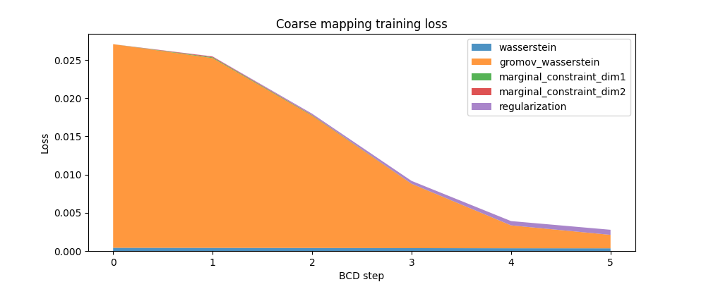
Here is the evolution of the FUGW loss during training of the coarse mapping, as well as the contribution of each loss term:

fig, ax = plt.subplots(figsize=(10, 4))
ax.set_title("Coarse mapping training loss")
ax.set_ylabel("Loss")
ax.set_xlabel("BCD step")
ax.stackplot(
    coarse_mapping.loss_steps,
    [
        (1 - alpha_coarse) * np.array(coarse_mapping.loss["wasserstein"]),
        alpha_coarse * np.array(coarse_mapping.loss["gromov_wasserstein"]),
        rho_coarse * np.array(coarse_mapping.loss["marginal_constraint_dim1"]),
        rho_coarse * np.array(coarse_mapping.loss["marginal_constraint_dim2"]),
        eps_coarse * np.array(coarse_mapping.loss["regularization"]),
    ],
    labels=[
        "wasserstein",
        "gromov_wasserstein",
        "marginal_constraint_dim1",
        "marginal_constraint_dim2",
        "regularization",
    ],
    alpha=0.8,
)
ax.legend()
plt.show()

And here is a similar plot for the fine-grained mapping:

fig, ax = plt.subplots(figsize=(10, 4))
ax.set_title("Fine-grained mapping training loss")
ax.set_ylabel("Loss")
ax.set_xlabel("BCD step")
ax.stackplot(
    fine_mapping.loss_steps,
    [
        (1 - alpha_fine) * np.array(fine_mapping.loss["wasserstein"]),
        alpha_fine * np.array(fine_mapping.loss["gromov_wasserstein"]),
        rho_fine * np.array(fine_mapping.loss["marginal_constraint_dim1"]),
        rho_fine * np.array(fine_mapping.loss["marginal_constraint_dim2"]),
        eps_fine * np.array(fine_mapping.loss["regularization"]),
    ],
    labels=[
        "wasserstein",
        "gromov_wasserstein",
        "marginal_constraint_dim1",
        "marginal_constraint_dim2",
        "regularization",
    ],
    alpha=0.8,
)
ax.legend()
plt.show()

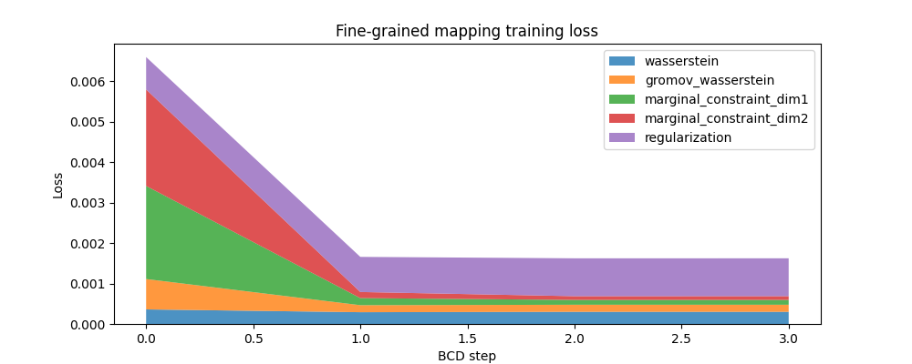
Note how few iterations are needed for the fine-grained model to converge compared to the coarse one, although the coarse model usually runs much faster (in total time) than the fine-grained one. It probably is a good strategy to invest computational time in deriving a precise coarse solution.

print(f"Total training time: {t1 - t0:.1f}s")

Total training time: 105.0s

Using the computed mappings

In this example, the transport plan of the coarse mapping is already too big to be displayed, but we can still look at the top-left corder. This plot will not always be informative, as mapped vertices are sampled at random. In this example, it does show some structure though, due to the fact that the source and target meshes are the same, and that our uniform sampling strategy returns compable results for the 2 distributions.

coarse_pi = coarse_mapping.pi.numpy()
fig, ax = plt.subplots(figsize=(10, 10))
ax.set_title("Coarse transport plan (top-left corner)", fontsize=20)
ax.set_xlabel("target vertices", fontsize=15)
ax.set_ylabel("source vertices", fontsize=15)
im = plt.imshow(coarse_pi[:200, :200], cmap="viridis")
plt.colorbar(im, ax=ax, shrink=0.8)
plt.show()

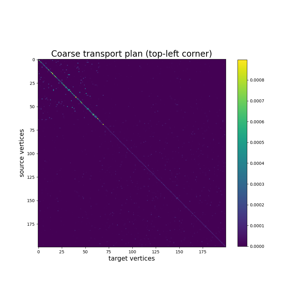
However, we can visualize the sparse transport plan computed by the fine-grained mapping, which is much more informative. Indeed, it exhibits some structure because the source and target meshes are the same: indeed, assuming vertex correspondence between the source and target mesh should already yield a reasonable alignment, we expected the diagonal of this matrix to be non-null.

indices = fine_mapping.pi.indices()
fine_mapping_as_scipy_coo = coo_matrix(
    (
        fine_mapping.pi.values(),
        (indices[0], indices[1]),
    ),
    shape=fine_mapping.pi.size(),
)

fig, ax = plt.subplots(figsize=(10, 10))
ax.set_title("Sparsity mask of fine-grained mapping", fontsize=15)
ax.set_ylabel("Source vertices", fontsize=15)
ax.set_xlabel("Target vertices", fontsize=15)
plt.spy(fine_mapping_as_scipy_coo, precision="present", markersize=0.01)
plt.show()

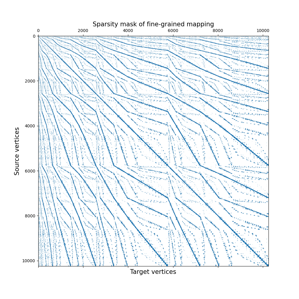
In this example, the computed sparse transport plan is quite sparse: it stores about 0.5% of what the equivalent dense transport plan would store.

100 * fine_mapping.pi.values().shape[0] / fine_mapping.pi.shape.numel()

1.1036252126387545

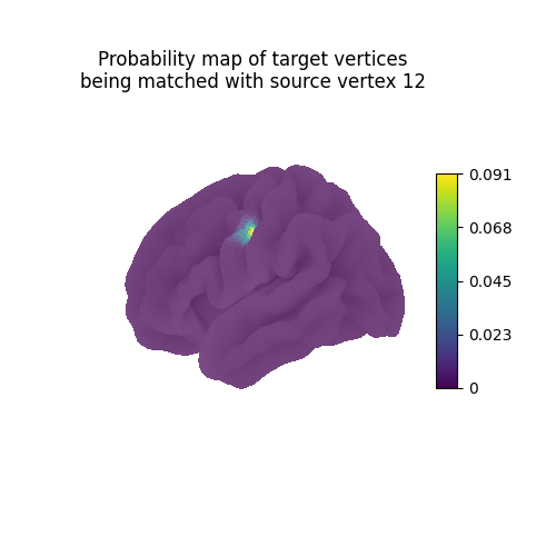
Each line vertex_index of the computed mapping can be interpreted as a probability map describing which vertices of the target should be mapped with the source vertex vertex_index. Since the ith row of a sparse matrix is not always easy to access, we fetch it by using .inverse_transform() on a one-hot vertor whose only non-null coefficient is at position vertex_index.

one_hot = np.zeros(source_features.shape[1])
one_hot[vertex_index] = 1.0
probability_map = fine_mapping.inverse_transform(one_hot)


fig = plt.figure(figsize=(5, 5))
ax = fig.add_subplot(111, projection="3d")
ax.set_title(
    "Probability map of target vertices\n"
    f"being matched with source vertex {vertex_index}"
)
plot_surface_map(probability_map, cmap="viridis", axes=ax)
plt.show()

Using mapping.transform(), we can use the computed mapping to transport any collection of feature maps from the source anatomy onto the target anatomy. Note that, conversely, mapping.inverse_transform() takes feature maps from the target anatomy and transports them on the source anatomy.

contrast_index = 2
predicted_target_features = fine_mapping.transform(
    source_features[contrast_index, :]
)
predicted_target_features.shape

(10242,)

fig = plt.figure(figsize=(3 * 3, 3))
fig.suptitle("Transporting feature maps of the training set")
grid_spec = gridspec.GridSpec(1, 3, figure=fig)

ax = fig.add_subplot(grid_spec[0, 0], projection="3d")
ax.set_title("Actual source features")
plot_surface_map(
    source_features[contrast_index, :], axes=ax, vmax=10, vmin=-10
)

ax = fig.add_subplot(grid_spec[0, 1], projection="3d")
ax.set_title("Predicted target features")
plot_surface_map(predicted_target_features, axes=ax, vmax=10, vmin=-10)

ax = fig.add_subplot(grid_spec[0, 2], projection="3d")
ax.set_title("Actual target features")
plot_surface_map(
    target_features[contrast_index, :], axes=ax, vmax=10, vmin=-10
)

plt.show()

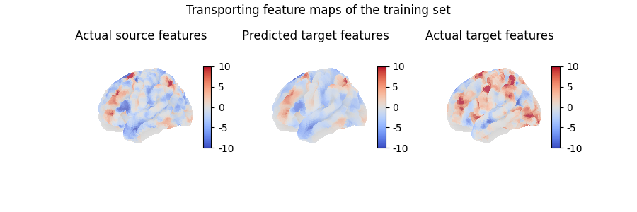
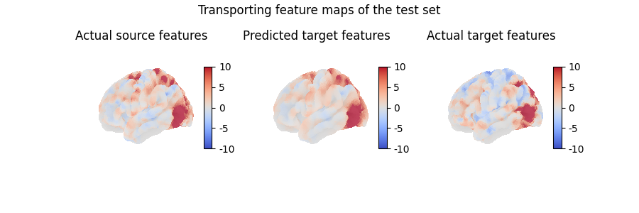
Here, we transported a feature map which is part of the traning set, which does not really help evaluate the quality of our model. Instead, we can also use the computed mapping to transport unseen data, which is how we will usually assess whether our model has captured useful information or not:

contrast_index = len(contrasts) - 1
predicted_target_features = fine_mapping.transform(
    source_features[contrast_index, :]
)

fig = plt.figure(figsize=(3 * 3, 3))
fig.suptitle("Transporting feature maps of the test set")
grid_spec = gridspec.GridSpec(1, 3, figure=fig)

ax = fig.add_subplot(grid_spec[0, 0], projection="3d")
ax.set_title("Actual source features")
plot_surface_map(
    source_features[contrast_index, :], axes=ax, vmax=10, vmin=-10
)

ax = fig.add_subplot(grid_spec[0, 1], projection="3d")
ax.set_title("Predicted target features")
plot_surface_map(predicted_target_features, axes=ax, vmax=10, vmin=-10)

ax = fig.add_subplot(grid_spec[0, 2], projection="3d")
ax.set_title("Actual target features")
plot_surface_map(
    target_features[contrast_index, :], axes=ax, vmax=10, vmin=-10
)

plt.show()

We can also partially transport feature maps, by specifying a parameter id_reg which balances the amount of regularization applied between the transport plan and the identity mapping. The regularized transport plan is then id_reg times the identity plus (1 - id_reg) times the transport plan computed by FUGW.

# Set of weights for the regularization parameter
id_reg = [0.0, 0.5, 1.0]

fig = plt.figure(figsize=(3 * 5, 4))
fig.suptitle(
    "Partial transportation of the feature maps by\nregularizing the transport"
    " plan with the identity"
)
grid_spec = gridspec.GridSpec(1, 5, figure=fig)

ax = fig.add_subplot(grid_spec[0, 0], projection="3d")
ax.set_title("Actual source features")
plot_surface_map(
    source_features[contrast_index, :],
    axes=ax,
    vmax=10,
    vmin=-10,
    colorbar=False,
)

for i, weight in enumerate(sorted(id_reg, reverse=True)):
    predicted_target_features = fine_mapping.transform(
        source_features[contrast_index, :],
        id_reg=weight,
    )
    ax = fig.add_subplot(grid_spec[0, i + 1], projection="3d")
    ax.set_title(f"id_reg={weight}")
    plot_surface_map(
        predicted_target_features, axes=ax, vmax=10, vmin=-10, colorbar=False
    )

ax = fig.add_subplot(grid_spec[0, -1], projection="3d")
ax.set_title("Actual target features")
plot_surface_map(
    target_features[contrast_index, :],
    axes=ax,
    vmax=10,
    vmin=-10,
    colorbar=False,
)

plt.show()

Estimated memory usage: 680 MB