Low-resolution surface alignment of 2 individuals with fMRI data

In this example, we align 2 low-resolution left hemispheres using 4 fMRI feature maps (z-score contrast maps).

import gdist
import matplotlib as mpl
import matplotlib.gridspec as gridspec
import matplotlib.pyplot as plt
import numpy as np

from fugw.mappings import FUGW
from fugw.utils import load_mapping, save_mapping
from mpl_toolkits.axes_grid1 import make_axes_locatable
from nilearn import datasets, image, plotting, surface

Let’s download 5 volumetric contrast maps per individual using nilearn’s API. We will use the first 4 of them to compute an alignment between the source and target subjects, and use the left-out contrast to assess the quality of our alignment.

n_subjects = 2

contrasts = [
    "sentence reading vs checkerboard",
    "sentence listening",
    "calculation vs sentences",
    "left vs right button press",
    "checkerboard",
]
n_training_contrasts = 4

brain_data = datasets.fetch_localizer_contrasts(
    contrasts,
    n_subjects=n_subjects,
    get_anats=True,
)

source_imgs_paths = brain_data["cmaps"][0 : len(contrasts)]
target_imgs_paths = brain_data["cmaps"][len(contrasts) : 2 * len(contrasts)]

Dataset created in /github/home/nilearn_data/brainomics_localizer

Downloading data from https://osf.io/hwbm2/download ...
 ...done. (2 seconds, 0 min)
Downloading data from https://osf.io/download/5d27cd441c5b4a001aa08008/ ...
 ...done. (3 seconds, 0 min)
Downloading data from https://osf.io/download/5d27c03e45253a001c3e189f/ ...
 ...done. (2 seconds, 0 min)
Downloading data from https://osf.io/download/5d27bfd0114a420016057cba/ ...
 ...done. (2 seconds, 0 min)
Downloading data from https://osf.io/download/5d27cb281c5b4a001aa07e29/ ...
 ...done. (2 seconds, 0 min)
Downloading data from https://osf.io/download/5d27cc0845253a001c3e22bd/ ...
 ...done. (2 seconds, 0 min)
Downloading data from https://osf.io/download/5d27d10b114a420019044ed8/ ...
 ...done. (3 seconds, 0 min)
Downloading data from https://osf.io/download/5d27d89d1c5b4a001d9f5e6e/ ...
 ...done. (2 seconds, 0 min)
Downloading data from https://osf.io/download/5d27d429a26b340017083380/ ...
 ...done. (2 seconds, 0 min)
Downloading data from https://osf.io/download/5d27ddc91c5b4a001b9ef9d0/ ...
 ...done. (2 seconds, 0 min)
Downloading data from https://osf.io/download/5d27d14f114a420019044efc/ ...
 ...done. (3 seconds, 0 min)
Downloading data from https://osf.io/download/5d275eb845253a001c3dbf76/ ...

Downloaded 3940352 of 14012301 bytes (28.1%,    2.6s remaining) ...done. (3 seconds, 0 min)
Downloading data from https://osf.io/download/5d275ede1c5b4a001aa00c26/ ...

Downloaded 5439488 of 13951266 bytes (39.0%,    1.6s remaining) ...done. (3 seconds, 0 min)
Downloading data from https://osf.io/download/5d27037f45253a001c3d4563/ ...
 ...done. (2 seconds, 0 min)
Downloading data from https://osf.io/download/5d7b8948fcbf44001c44e695/ ...
 ...done. (2 seconds, 0 min)

Here is what the first contrast map of the source subject looks like (the following figure is interactive):

contrast_index = 0
plotting.view_img(
    source_imgs_paths[contrast_index],
    brain_data["anats"][0],
    title=f"Contrast {contrast_index} (source subject)",
    opacity=0.5,
)

/usr/local/lib/python3.8/site-packages/nilearn/plotting/html_stat_map.py:198: UserWarning:

Non-finite values detected. These values will be replaced with zeros.

/usr/local/lib/python3.8/site-packages/numpy/core/fromnumeric.py:784: UserWarning:

Warning: 'partition' will ignore the 'mask' of the MaskedArray.

Computing feature arrays

Let’s project these 4 maps to a mesh representing the cortical surface and aggregate these projections to build an array of features for the source and target subjects. For the sake of keeping the training phase of our mapping short even on CPU, we project these volumetric maps on a very low-resolution mesh made of 642 vertices.

fsaverage3 = datasets.fetch_surf_fsaverage(mesh="fsaverage3")

def load_images_and_project_to_surface(image_paths):
    """Util function for loading and projecting volumetric images."""
    images = [image.load_img(img) for img in image_paths]
    surface_images = [
        np.nan_to_num(surface.vol_to_surf(img, fsaverage3.pial_left))
        for img in images
    ]

    return np.stack(surface_images)


source_features = load_images_and_project_to_surface(source_imgs_paths)
target_features = load_images_and_project_to_surface(target_imgs_paths)
source_features.shape

/usr/local/lib/python3.8/site-packages/nilearn/surface/surface.py:464: RuntimeWarning:

Mean of empty slice

/usr/local/lib/python3.8/site-packages/nilearn/surface/surface.py:464: RuntimeWarning:

Mean of empty slice

/usr/local/lib/python3.8/site-packages/nilearn/surface/surface.py:464: RuntimeWarning:

Mean of empty slice

/usr/local/lib/python3.8/site-packages/nilearn/surface/surface.py:464: RuntimeWarning:

Mean of empty slice

/usr/local/lib/python3.8/site-packages/nilearn/surface/surface.py:464: RuntimeWarning:

Mean of empty slice

/usr/local/lib/python3.8/site-packages/nilearn/surface/surface.py:464: RuntimeWarning:

Mean of empty slice

/usr/local/lib/python3.8/site-packages/nilearn/surface/surface.py:464: RuntimeWarning:

Mean of empty slice

/usr/local/lib/python3.8/site-packages/nilearn/surface/surface.py:464: RuntimeWarning:

Mean of empty slice

/usr/local/lib/python3.8/site-packages/nilearn/surface/surface.py:464: RuntimeWarning:

Mean of empty slice

/usr/local/lib/python3.8/site-packages/nilearn/surface/surface.py:464: RuntimeWarning:

Mean of empty slice


(5, 642)

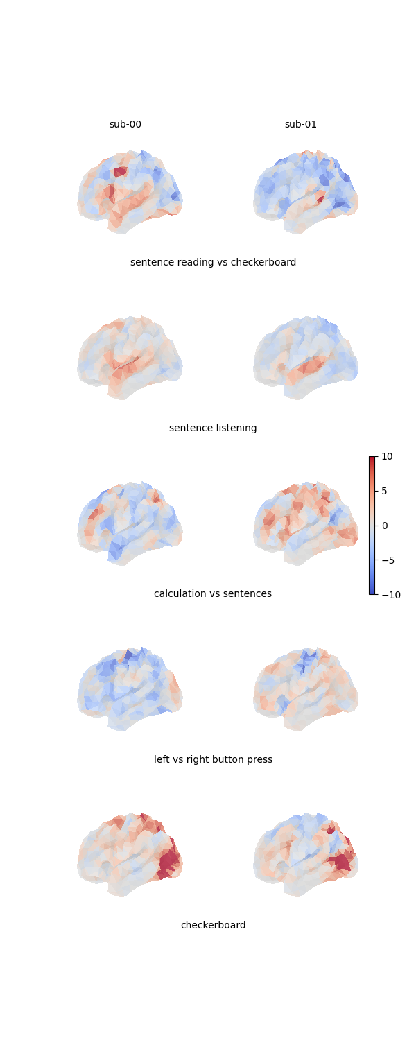
Here is a figure showing the 4 projected maps for each of the 2 individuals:

def plot_surface_map(surface_map, cmap="coolwarm", colorbar=True, **kwargs):
    """Util function for plotting surfaces."""
    plotting.plot_surf(
        fsaverage3.pial_left,
        surface_map,
        cmap=cmap,
        colorbar=colorbar,
        bg_map=fsaverage3.sulc_left,
        bg_on_data=True,
        darkness=0.5,
        **kwargs,
    )


fig = plt.figure(figsize=(3 * n_subjects, 3 * len(contrasts)))
grid_spec = gridspec.GridSpec(len(contrasts), n_subjects, figure=fig)

# Print all feature maps
for i, contrast_name in enumerate(contrasts):
    for j, features in enumerate([source_features, target_features]):
        ax = fig.add_subplot(grid_spec[i, j], projection="3d")
        plot_surface_map(
            features[i, :], axes=ax, vmax=10, vmin=-10, colorbar=False
        )

    # Add labels to subplots
    if i == 0:
        for j in range(2):
            ax = fig.add_subplot(grid_spec[i, j])
            ax.axis("off")
            ax.text(0.5, 1, f"sub-0{j}", va="center", ha="center")

    ax = fig.add_subplot(grid_spec[i, :])
    ax.axis("off")
    ax.text(0.5, 0, contrast_name, va="center", ha="center")

# Add colorbar
ax = fig.add_subplot(grid_spec[2, :])
ax.axis("off")
divider = make_axes_locatable(ax)
cax = divider.append_axes("right", size="2%")
fig.add_axes(cax)
fig.colorbar(
    mpl.cm.ScalarMappable(
        norm=mpl.colors.Normalize(vmin=-10, vmax=10), cmap="coolwarm"
    ),
    cax=cax,
)

plt.show()

Computing geometry arrays

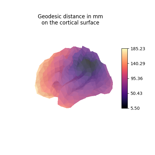
Now we compute the kernel matrix of distances between vertices on the cortical surface. Note that in this example, we are using the same mesh for the source and target individuals, but this does not have to be the case in general.

def compute_geometry_from_mesh(mesh_path):
    """Util function to compute matrix of geodesic distances of a mesh."""
    (coordinates, triangles) = surface.load_surf_mesh(mesh_path)
    geometry = gdist.local_gdist_matrix(
        coordinates.astype(np.float64), triangles.astype(np.int32)
    ).toarray()

    return geometry


fsaverage3_pial_left_geometry = compute_geometry_from_mesh(
    fsaverage3.pial_left
)
source_geometry = fsaverage3_pial_left_geometry
target_geometry = fsaverage3_pial_left_geometry
source_geometry.shape

(642, 642)

Each line vertex_index of the geometry matrices contains the anatomical distance (here in millimeters) from vertex_index to all other vertices of the mesh.

vertex_index = 4

fig = plt.figure(figsize=(5, 5))
ax = fig.add_subplot(111, projection="3d")
ax.set_title("Geodesic distance in mm\non the cortical surface")
plot_surface_map(
    source_geometry[vertex_index, :],
    cmap="magma",
    cbar_tick_format="%.2f",
    axes=ax,
)
plt.show()

Normalizing features and geometries

Features and geometries should be normalized before we can train a mapping. Indeed, without this scaling, it’s unclear whether the source and target features would be comparable. Moreover, the hyper-parameter alpha would depend on the scale of the respective matrices. Finally, it can empirically lead to having nan values in the computed transport plan.

source_features_normalized = source_features / np.linalg.norm(
    source_features, axis=1
).reshape(-1, 1)
target_features_normalized = target_features / np.linalg.norm(
    target_features, axis=1
).reshape(-1, 1)
source_geometry_normalized = source_geometry / np.max(source_geometry)
target_geometry_normalized = target_geometry / np.max(target_geometry)

Training the mapping

Let’s create our mapping. We set alpha=0.5 to indicate that we are as interested in matching vertices with similar features as we are in preserving the anatomical geometries of the source and target subjects. We leave rho to its default value, and finally set a value of eps which is low enough for the computed transport plan to not be too regularized. High values of eps lead to faster computations and more regularized (ie blurry) plans. Low values of eps lead to solwer computations, but finer-grained plans. Note that this package is meant to be used with GPUs ; fitting mappings on CPUs in about 100x slower.

alpha = 0.5
rho = 1
eps = 1e-4
mapping = FUGW(alpha=alpha, rho=rho, eps=eps)

Let’s fit our mapping! 🚀

Remember to use the training maps only. Moreover, we limit the number of block-coordinate-descent iterations to 3 in order to limit computation time for this example.

_ = mapping.fit(
    source_features_normalized[:n_training_contrasts],
    target_features_normalized[:n_training_contrasts],
    source_geometry=source_geometry_normalized,
    target_geometry=target_geometry_normalized,
    solver="sinkhorn",
    solver_params={
        "nits_bcd": 3,
    },
    verbose=True,
)

[15:43:42] Validation data for feature maps is not provided. Using  dense.py:199
           training data instead.
           Validation data for anatomical kernels is not provided.  dense.py:226
           Using training data instead.


[15:43:51] BCD step 1/3    FUGW loss:      0.029781434684991837     dense.py:568
           Validation loss:        0.029781434684991837


[15:44:06] BCD step 2/3    FUGW loss:      0.0056222956627607346    dense.py:568
           Validation loss:        0.0056222956627607346


[15:44:21] BCD step 3/3    FUGW loss:      0.005595004186034203     dense.py:568
           Validation loss:        0.005595004186034203

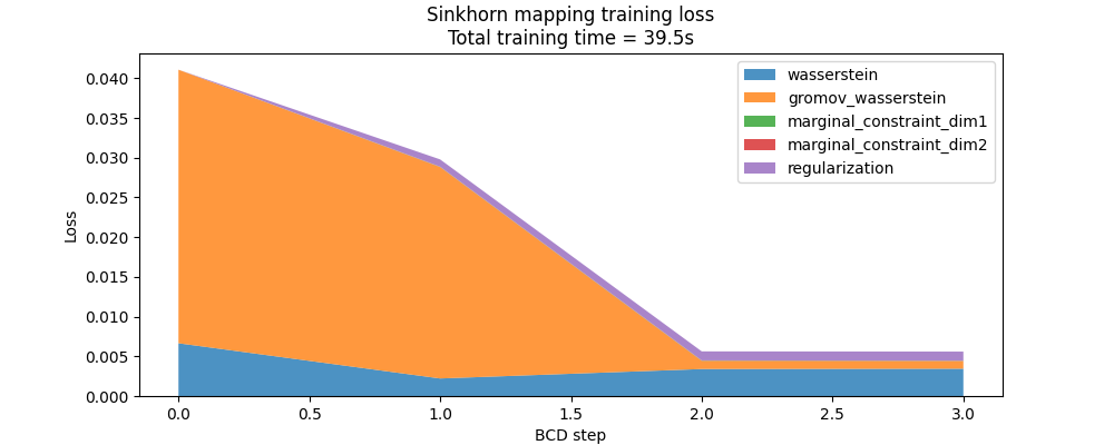
Here is the evolution of the FUGW loss during training, with and without the regularized term:

fig, ax = plt.subplots(figsize=(10, 4))
ax.set_title(
    "Sinkhorn mapping training loss\n"
    f"Total training time = {mapping.loss_times[-1]:.1f}s"
)
ax.set_ylabel("Loss")
ax.set_xlabel("BCD step")
ax.stackplot(
    mapping.loss_steps,
    [
        (1 - alpha) * np.array(mapping.loss["wasserstein"]),
        alpha * np.array(mapping.loss["gromov_wasserstein"]),
        rho * np.array(mapping.loss["marginal_constraint_dim1"]),
        rho * np.array(mapping.loss["marginal_constraint_dim2"]),
        eps * np.array(mapping.loss["regularization"]),
    ],
    labels=[
        "wasserstein",
        "gromov_wasserstein",
        "marginal_constraint_dim1",
        "marginal_constraint_dim2",
        "regularization",
    ],
    alpha=0.8,
)
ax.legend()
plt.show()

Note that we used the sinkhorn solver here because it’s well known in the optimal transport community, but that this library comes with other solvers which are, in most cases, much faster. Let’s retrain our mapping using the mm solver, which implements a maximize-minimization approach to approximate a solution and is used by default in fugw.mappings:

mm_mapping = FUGW(alpha=alpha, rho=rho, eps=eps)

_ = mm_mapping.fit(
    source_features_normalized[:n_training_contrasts],
    target_features_normalized[:n_training_contrasts],
    source_geometry=source_geometry_normalized,
    target_geometry=target_geometry_normalized,
    solver="mm",
    solver_params={
        "nits_bcd": 5,
        "tol_bcd": 1e-10,
        "tol_uot": 1e-10,
    },
    verbose=True,
)

[15:44:22] Validation data for feature maps is not provided. Using  dense.py:199
           training data instead.
           Validation data for anatomical kernels is not provided.  dense.py:226
           Using training data instead.


[15:44:24] BCD step 1/5    FUGW loss:      0.03694058209657669      dense.py:568
           Validation loss:        0.03694058209657669


[15:44:27] BCD step 2/5    FUGW loss:      0.01503392867743969      dense.py:568
           Validation loss:        0.01503392867743969


[15:44:29] BCD step 3/5    FUGW loss:      0.0076630255207419395    dense.py:568
           Validation loss:        0.0076630255207419395


[15:44:32] BCD step 4/5    FUGW loss:      0.006633032578974962     dense.py:568
           Validation loss:        0.006633032578974962


[15:44:36] BCD step 5/5    FUGW loss:      0.006219181232154369     dense.py:568
           Validation loss:        0.006219181232154369

And now with the ibpp solver:

ibpp_mapping = FUGW(alpha=alpha, rho=rho, eps=eps)

_ = ibpp_mapping.fit(
    source_features_normalized[:n_training_contrasts],
    target_features_normalized[:n_training_contrasts],
    source_geometry=source_geometry_normalized,
    target_geometry=target_geometry_normalized,
    solver="ibpp",
    solver_params={
        "nits_bcd": 5,
        "tol_bcd": 1e-10,
        "tol_uot": 1e-10,
    },
    verbose=True,
)

           Validation data for feature maps is not provided. Using  dense.py:199
           training data instead.
           Validation data for anatomical kernels is not provided.  dense.py:226
           Using training data instead.


[15:44:38] BCD step 1/5    FUGW loss:      0.034542761743068695     dense.py:568
           Validation loss:        0.034542761743068695


[15:44:41] BCD step 2/5    FUGW loss:      0.0077322423458099365    dense.py:568
           Validation loss:        0.0077322423458099365


[15:44:44] BCD step 3/5    FUGW loss:      0.00618749251589179      dense.py:568
           Validation loss:        0.00618749251589179


[15:44:48] BCD step 4/5    FUGW loss:      0.005864568054676056     dense.py:568
           Validation loss:        0.005864568054676056


[15:44:53] BCD step 5/5    FUGW loss:      0.005737483035773039     dense.py:568
           Validation loss:        0.005737483035773039

Computed mappings can easily be saved on disk and loaded back. Note that fugw.mappings overwrite functions used by pickle so that hyper-parameters and model weights are stored separately. This is handy if you want to quickly load a mapping without its weights.

# Save mappings
save_mapping(mapping, "./mapping.pkl")

# Load mappings
mapping = load_mapping("./mapping.pkl")
# Load mappings hyper-parameters only
mapping_without_weights = load_mapping("./mapping.pkl", load_weights=False)

print(f"With weights: pi = tensor of size {mapping.pi.shape}")
print(f"Without weights: pi = {mapping_without_weights.pi}")

           FUGW customizes pickle dumps to separate hyperparams and  utils.py:90
           weights. Please check the documentation.
           FUGW customizes pickle dumps to separate hyperparams and  utils.py:99
           weights. Please check the documentation.
           FUGW customizes pickle dumps to separate hyperparams and  utils.py:99
           weights. Please check the documentation.
With weights: pi = tensor of size torch.Size([642, 642])
Without weights: pi = None

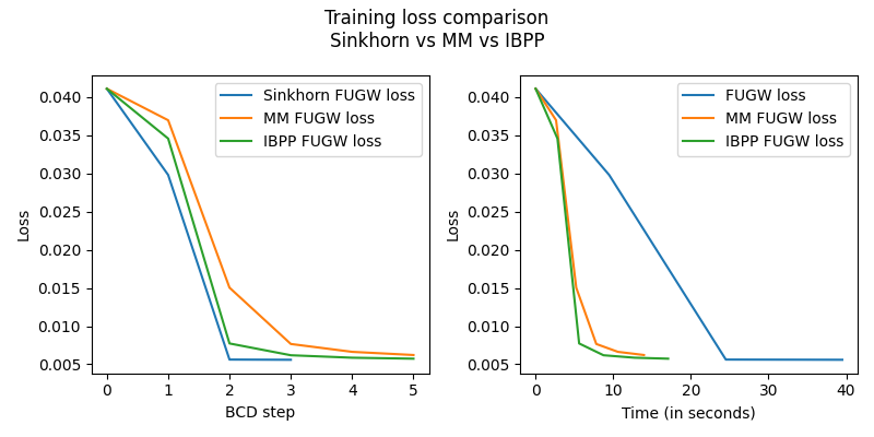
Here is the evolution of the FUGW loss during training, without the regularized term. Note how, in this case, even though mm and ibpp needed more block-coordinate-descent steps to converge, they were about 2 to 3 times faster to reach the same final FUGW training loss as sinkhorn. You might want to tweak solver parameters like nits_bcd and nits_uot to get the fastest convergence rates.

fig = plt.figure(figsize=(4 * 2, 4))
fig.suptitle("Training loss comparison\nSinkhorn vs MM vs IBPP")

ax = fig.add_subplot(121)
ax.set_ylabel("Loss")
ax.set_xlabel("BCD step")
ax.plot(mapping.loss_steps, mapping.loss["total"], label="Sinkhorn FUGW loss")
ax.plot(mm_mapping.loss_steps, mm_mapping.loss["total"], label="MM FUGW loss")
ax.plot(
    ibpp_mapping.loss_steps, ibpp_mapping.loss["total"], label="IBPP FUGW loss"
)
ax.legend()

ax = fig.add_subplot(122)
ax.set_ylabel("Loss")
ax.set_xlabel("Time (in seconds)")
ax.plot(mapping.loss_times, mapping.loss["total"], label="FUGW loss")
ax.plot(mm_mapping.loss_times, mm_mapping.loss["total"], label="MM FUGW loss")
ax.plot(
    ibpp_mapping.loss_times, ibpp_mapping.loss["total"], label="IBPP FUGW loss"
)
ax.legend()

fig.tight_layout()
plt.show()

Using the computed mapping

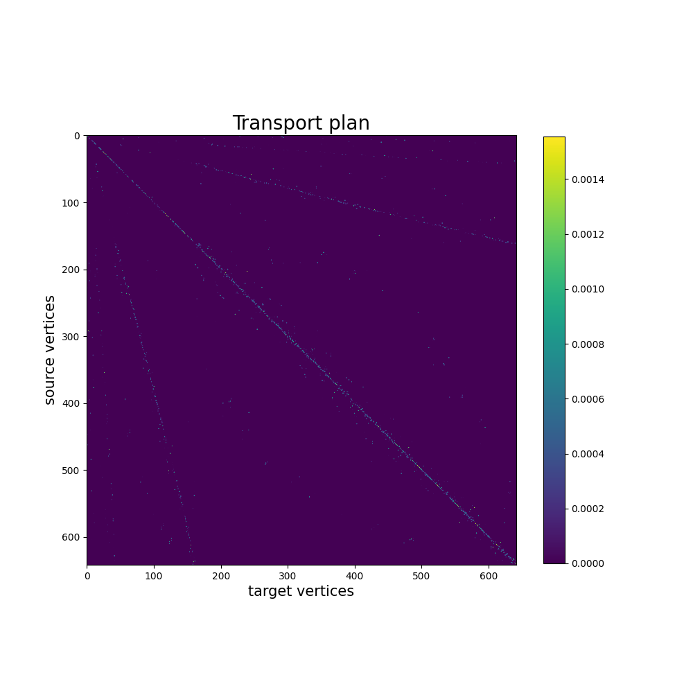
The computed mapping is stored in mapping.pi as a torch.Tensor. In this example, the transport plan is small enough that we can display it altogether.

pi = mapping.pi.numpy()
fig, ax = plt.subplots(figsize=(10, 10))
ax.set_title("Transport plan", fontsize=20)
ax.set_xlabel("target vertices", fontsize=15)
ax.set_ylabel("source vertices", fontsize=15)
im = plt.imshow(pi, cmap="viridis")
plt.colorbar(im, ax=ax, shrink=0.8)
plt.show()

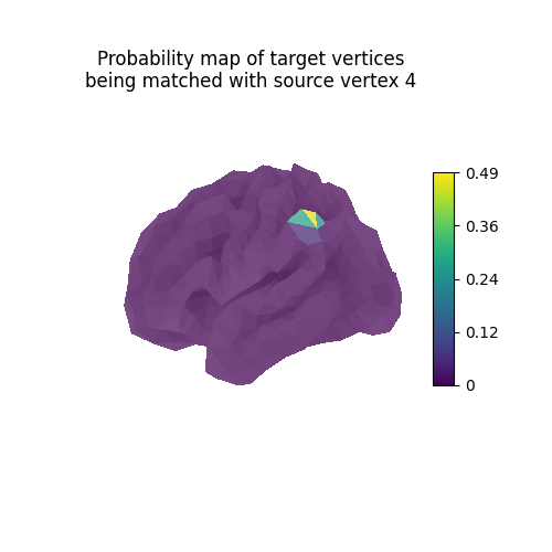
Each line vertex_index of the computed mapping can be interpreted as a probability map describing which vertices of the target should be mapped with the source vertex vertex_index.

probability_map = pi[vertex_index, :] / np.linalg.norm(pi[vertex_index, :])

fig = plt.figure(figsize=(5, 5))
ax = fig.add_subplot(111, projection="3d")
ax.set_title(
    "Probability map of target vertices\n"
    f"being matched with source vertex {vertex_index}"
)
plot_surface_map(probability_map, cmap="viridis", axes=ax)
plt.show()

Using mapping.transform(), we can use the computed mapping to transport any collection of feature maps from the source anatomy onto the target anatomy. Note that, conversely, mapping.inverse_transform() takes feature maps from the target anatomy and transports them on the source anatomy.

contrast_index = 2
predicted_target_features = mapping.transform(
    source_features[contrast_index, :]
)
predicted_target_features.shape

(642,)

fig = plt.figure(figsize=(3 * 3, 3))
fig.suptitle("Transporting feature maps of the training set")
grid_spec = gridspec.GridSpec(1, 3, figure=fig)

ax = fig.add_subplot(grid_spec[0, 0], projection="3d")
ax.set_title("Actual source features")
plot_surface_map(
    source_features[contrast_index, :], axes=ax, vmax=10, vmin=-10
)

ax = fig.add_subplot(grid_spec[0, 1], projection="3d")
ax.set_title("Predicted target features")
plot_surface_map(predicted_target_features, axes=ax, vmax=10, vmin=-10)

ax = fig.add_subplot(grid_spec[0, 2], projection="3d")
ax.set_title("Actual target features")
plot_surface_map(
    target_features[contrast_index, :], axes=ax, vmax=10, vmin=-10
)

plt.show()

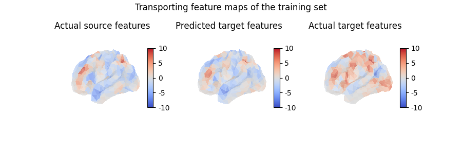
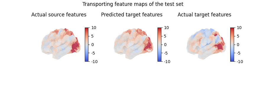
Here, we transported a feature map which is part of the traning set, which does not really help evaluate the quality of our model. Instead, we can also use the computed mapping to transport unseen data, which is how we will usually assess whether our model has captured useful information or not:

contrast_index = len(contrasts) - 1
predicted_target_features = mapping.transform(
    source_features[contrast_index, :]
)

fig = plt.figure(figsize=(3 * 3, 3))
fig.suptitle("Transporting feature maps of the test set")
grid_spec = gridspec.GridSpec(1, 3, figure=fig)

ax = fig.add_subplot(grid_spec[0, 0], projection="3d")
ax.set_title("Actual source features")
plot_surface_map(
    source_features[contrast_index, :], axes=ax, vmax=10, vmin=-10
)

ax = fig.add_subplot(grid_spec[0, 1], projection="3d")
ax.set_title("Predicted target features")
plot_surface_map(predicted_target_features, axes=ax, vmax=10, vmin=-10)

ax = fig.add_subplot(grid_spec[0, 2], projection="3d")
ax.set_title("Actual target features")
plot_surface_map(
    target_features[contrast_index, :], axes=ax, vmax=10, vmin=-10
)

plt.show()

Estimated memory usage: 302 MB